Many articles explaining I/Q signals start off with the theory and follow up with practical applications. While that is a valid approach to the topic, it often does not convey the reason for their usefulness. I want to address that by working backwards, from the issue to the solution, by analyzing a frequent use case of I/Q signals: RF transmission and reception.

Bear in mind that throughout the article I will be simplifying (and sometimes oversimplifying) some concepts, I will tacitly make some nontrivial assumptions (like oscillator phase synchronization) and sometimes the math will not be very rigurous.

This article is meant to give a deep intuition on the topic, not to be used as a textbook.

From sound to aether

Let’s consider a continuous and time-variant baseband signal, the voltage transduced by a microphone from sound waves. From Fourier analysis we know that we can express any such signal as a finite or infinite sum of simple trigonometric functions:

$$ x(t) = \sum_{k} A_k \cos (2 \pi t f_k + \phi_k) $$

Each term of the sum is a sinusoid characterized by an amplitude \(A_k\), a frequency \(f_k\) and a phase \(\phi_k\).

Since we are dealing with voice, we can assume that \( f_k \lt 4\text{kHz} \) which means that our signal \(x\) has a bandwidth of \(4\text{kHz}\).

Simple is not necessarily better

The most straightforward way to transmit this signal would be to connect the microphone output to a high gain amplifier and connect the amplifier to an antenna.

However, this raises some very important issues. Since at these frequencies the wavelengths are on the order of tens to thousands of kilometers, the antenna would need to be impractically large and will have low efficiency. As a consequence, the transmission power needs to be, again, impractically large.

Also, because all humans share virtually the same vocal range, the channel would be highly susceptible to interference; imagine trying to talk to somebody across a crowded room when everybody else is trying to do the same.

In order to solve the first problem, the solution is to somehow translate the signal into a higher frequency band, where antennas are smaller and power requirements are reasonable. Also, to mitigate the issue of interference, it would be nice to be able to finely control the target frequency band, so as to avoid transmitting over other people’s signals.

This is exactly what modern RF transceivers do, and to understand how we need a bit more math.

The frequency mixer

Let’s consider another signal \(c\) of frequency \(f_c\), which we will call the carrier signal or carrier wave.

$$ c(t) = \cos (2 \pi t f_c) $$

Amplitude modulation is the process of controlling a carrier wave’s amplitude using the baseband signal. This translates to multiplying two signals together into a third signal \(y\).

$$ \begin{align} y(t) & = x(t) c(t) \\ & = \sum_{k} A_k \cos (2 \pi t f_k + \phi_k) \cos (2 \pi t f_c) \end{align} $$

Given the trigonometric identity

$$ \cos(a) \cos(b) = \frac{1}{2} \left[ \cos(a+b) + cos(a-b) \right] $$

we can write \(y\) as

$$ \begin{align} y(t) & = \sum_{k} A_k \frac{1}{2} \left[ \cos (2 \pi t (f_c + f_k) + \phi_k ) + \cos (2 \pi t (f_c - f_k) - \phi_k) \right] \\ & = \frac{1}{2} \sum_{k} A_k \cos (2 \pi t (f_c + f_k) + \phi_k) + \frac{1}{2} \sum_{k} A_k \cos (2 \pi t (f_c - f_k) - \phi_k) \end{align} $$

What the above result tells us is that signal multiplication shifts each component of frequency \(f_k\) from the original signal into two components at \(f_c+f_k\) and \(f_c-f_k\), each carrying half the energy of the original, thus behaving as a frequency mixer

For example, if we have a carrier wave of \(f_c=7\text{MHz}\) and \(x\) is a pure \(1\text{kHz}\) tone, then \(y\) will exhibit two equally energetic components at \(6.999\text{MHz}\) and \(7.001\text{MHz}\). This new signal is much more fit for RF transmission than the baseband signal; a well built \(10m\) antenna and \(100W\) of power can potentially carry the signal around the world.

The case of negative frequencies

A very obvious question is why have we chosen \(f_c-f_k\) instead of \(f_k-f_c\). The answer is quite simple - since the cosine is an even function it doesn’t matter. Thus, \( \cos(a) = \cos(-a) \), so regardless of which frequency we subtract from which, the result is identical.

This raises a crucial point: when dealing with real signals, the concept of negative frequencies is irrelevant. We can express them mathematically, but when it comes to their realization they always alias to the same waveform of their positive counterparts.

Signal recovery

How do we recover our signal \(x\) from \(y\)? Well, it turns out that multiplying \(y\) again with the same carrier wave will yield the following mapping of component frequencies:

$$ \begin{align} (f_c-f_k) \mapsto & { f_c-(f_c-f_k), f_c+(f_c-f_k) } \\ (f_c+f_k) \mapsto & { f_c-(f_c+f_k), f_c+(f_c+f_k) } \end{align} $$

After simplification:

$$ \begin{align} (f_c-f_k) \mapsto & { f_k, 2 f_c-f_k } \\ (f_c+f_k) \mapsto & { f_k, 2 f_c+f_k } \end{align} $$

Thus, the product $$ \begin{align} z(t) & =y(t)c(t) \\ & = x(t)c(t)c(t) \\ & = \frac{1}{2}x(t) + \frac{1}{2} x(t) \cos (4 \pi t f_c) \end{align} $$

will contain \(x\) at half the original energy as well as the product of \(x\) with twice the carrier frequency. Since the latter is so far out of the audio spectrum, it is trivial to filter out, and thus recover \(x\) and feed it to some sort of output like a speaker.

Optimizing bandwidth usage

The above model describes a modulation called Double Sideband Suppressed Carrier Amplitude Modulation. Each of the mirrored versions of the shifted signal (above and below the carrier frequency) is called a sideband, hence the name.

However, it has an issue: while \(x\) has a bandwidth of \(4\text{kHz}\), \(y\) needs twice that because of the two sidebands (each \(4\text{kHz}\) wide). Since the two sidebands are redundant (i.e. they contain the same information), it is an unnecessary waste of bandwidth.

As a result, it is desired to arbitrarily suppress one of them (through filtration or phasing, although the former is quite difficult), yielding a signal containing only the lower or upper sideband. Intuitively, this is called Single Sideband Suppressed Carrier Amplitude Modulation.

If for example we chose to keep the upper sideband, the space just below the carrier frequency can now be used by another user without interfering with our transmission, thus effectively doubling the capacity of the band.

Image rejection issues

The above optimization raises an important issue. In the case of DSB-SC modulation we could filter unwanted signals after mixing.

We cannot use the same strategy in the case of SSB-SC modulation, since it will irreversibly blend our desired signal with adjacent signals during the mixing process.

The solution would be to filter out the desired signal from \(y\) before mixing.

However implementing filters with good selectivity at high frequencies is expensive and difficult, much more difficult than at baseband frequencies. This is an issue for both SSB signal recovery (i.e. receiver) as well as SSB signal generation (i.e. transmission).

Revisiting negative frequencies

Imagine there is a black box whose state \((f, \phi)\) encodes a frequency \(f\) and a phase \(\phi\), both of which can be positive or negative. We cannot look into the black box, but we can observe its output of unit amplitude \(\cos (2 \pi t f + \phi)\) over time.

However, since \(\cos\) is an even function, we have the equality:

$$ \cos (2 \pi t f + \phi) = \cos (-2 \pi t f - \phi) \text{, } \forall t,f,\phi \in \Bbb{R} $$

This means that if we try to reconstruct the waveform (through magic, hard work or math) we will reach two solutions:

$$ S = \Bigl \{ (f, \phi), (-f, -\phi) \Bigr \} $$

without being able to tell which is the correct one and which is the wrong one.

Now let’s say we add another output to our black box, which returns \(\cos (2 \pi t f + \phi + \theta)\), for some known \( \theta \in (-\pi, \pi) \text{, } \theta \ne 0 \).

If we now try to reconstruct this new waveform we will again reach two solutions:

$$ S_\theta = \Bigl \{ (f, \phi + \theta), (-f, -\phi - \theta) \Bigr \} $$

However, we know that these have a phase difference (in relation to \(S\)) of exactly \(\theta\), so we can build a new set of solutions for the first waveform by subtracting \(\theta\) from \(S_\theta\):

$$ \begin{align} S^\star & = \Bigl \{ (f, \phi + \theta - \theta), (-f, -\phi - \theta - \theta) \Bigr \} \\ & = \Bigl \{ (f, \phi), (-f, -\phi - 2 \theta) \Bigr \} \end{align} $$

Since \(\theta \ne 0\), the two sets will have only one solution in common, which is the state within the black box:

$$ S \cap S^\star = \Bigl \{ (f, \phi) \Bigr \} $$

What the above reasoning tells us is that if we have a signal and a version of this signal whose components are out of phase by some known \(\theta\), then we can discriminate between positive and negative frequencies. Let’s now see how we can pack them into a representation that is easier to work with.

If we choose \(\theta = -\frac{\pi}{2}\) then the out of phase waveform is

$$ \cos (2 \pi f t + \phi - \frac{\pi}{2}) = \sin (2 \pi f t + \phi) $$

Since

$$ \cos^2 (2 \pi f t + \phi) + \sin^2 (2 \pi f t + \phi) = 1 $$

it follows that the two waveforms describe a unit circle in a Cartesian coordinate system. Plotting \( \vec{v}(t) = \begin{bmatrix} \cos (2 \pi f t + \phi) \\ \sin (2 \pi f t + \phi) \end{bmatrix} \) will give us some intuition of what we have built so far:

While the projection of \(\vec{v}\) on the horisontal axis is identical in both plots (which was actually our issue from the beginning), we can now see an obvious difference between the two: for positive frequencies the vector rotates counterclockwise while for negative frequencies it rotates clockwise. This is due to the fact that, unlike \(\cos\), \(\sin\) is an odd function (i.e. \(\sin(-x)=-\sin(x)\)).

For brevity we call \(\cos (2 \pi f t + \phi)\) the in-phase or I component and \(\sin (2 \pi f t + \phi)\) the quadrature or Q component of the signal. Generally speaking, any two signals which are out of phase by \(\pm\frac{\pi}{2}\) are said to be orthogonal to each other, or in quadrature.

There is one more piece of intuition we can draw from this representation. Until now we have expressed any real signal as a function of time, amplitude, frequency and phase. Each of these four variables contribute in some way to the single output that is the instantaneous amplitude.

Now that we introduced the quadradure component, we have two such signals that are expressed as a function of the same four variables; while we solved our aliasing issue, we did not make our job easier in handling them.

However, if we consider \(\vec{v}\) in polar coordinates, we notice that the radial coordinate \(\rho\) is exactly equal to the amplitude, while the angular coordinate \(\Phi\) is a function of time, frequency and phase:

$$ \rho = |\vec{v}| = A \\ \Phi = 2 \pi f t + \phi $$

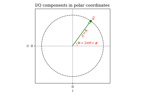
Moreover, the angular velocity is strictly a function of frequency:

$$ \frac{d \Phi}{dt} = 2 \pi f $$

Thus, for some sinusoid of fixed \((A, f, \phi)\), the in-phase and quadrature components describe an \(A\)-length vector rotating with a constant rate determined by \(|f|\) with the direction of rotation determined by the sign of \(f\).

Since this vector representation holds for addition (i.e. summing multiple sinusoids), we can plot part of our baseband signal over time:

Complex signals

Let’s consider writing the I and Q components as a complex number:

$$ v(t) = A \cos (2 \pi t f + \phi) + j A \sin (2 \pi t f + \phi) \\ \text{where } j^2 = -1 $$

We can easily observe that this complex representation holds for addition and multiplication with a real number, i.e. the operation result’s real and imaginary parts are still in quadrature.

However, something funny happens when we multiply two such complex sinusoid:

$$ (A_1 \cos \Phi_1 + j A_1 \sin \Phi_1) (A_2 \cos \Phi_2 + j A_2 \sin \Phi_2) \\ = A_1 A_2 \left[ \cos\Phi_1 \cos\Phi_2 + j^2 \sin\Phi_1 \sin\Phi_2 + j (\cos\Phi_1 \sin\Phi_2 + \sin\Phi_1 \cos\Phi_2) \right] \\ = A_1 A_2 \left[ (\cos\Phi_1 \cos\Phi_2 - \sin\Phi_1 \sin\Phi_2) + j (\cos\Phi_1 \sin\Phi_2 + \sin\Phi_1 \cos\Phi_2) \right] \\ = A_1 A_2 \left[ \cos(\Phi_1 + \Phi_2) + j \sin(\Phi_1 + \Phi_2) \right] $$

Besides the fact that the representation holds for multiplication we can see that, unlike in the case of multiplication of real sinusoids, the product is no longer a sum of two sinusoids. This behaviour is very intuitive once you understand the geometric interpretation of complex number multiplication.

In order to make our lives even easier, by using Euler’s formula we can write these waveforms as a complex exponential:

$$ v(t) = A \cos (2 \pi t f + \phi) + j A \sin (2 \pi t f + \phi) = A \cdot e^{j (2 \pi t f_k + \phi_k)} $$

Or, to simplify, if we consider the angular frequency \(\omega = 2 \pi f\) expressed in \(rad \cdot s^{-1}\):

$$ v(t) = A e^{j (\omega t + \phi)} $$

Mixing complex signals

Let us now consider the complex baseband signal:

$$ x^\star(t) = \sum_{k} A_k e^{j (\omega_k t + \phi_k)} \\ x(t) = \operatorname{Re} (x^\star(t)) $$

and the complex carrier wave:

$$ c^\star(t) = e^{j \omega_c t} $$

When we multiply the signal with the carrier in the complex domain

$$ \begin{align} y^\star(t) & = x^\star(t) c^\star(t) \\ & = \sum_{k} A_k e^{j (\omega_k t + \phi_k)} e^{j \omega_c t} \\ & = \sum_{k} A_k e^{j \left[ (\omega_k + \omega_c) t + \phi_k \right]} \end{align} $$

we notice that the product no longer splits the original signal into two sidebands of equal energy. Instead, it simply translates (in the frequency domain) the baseband signal by \(f_c\). Thus we no longer need filtering to remove the unwanted sideband.

On the other hand, multiplying \(y^\star\) with \(c^\star\) no longer yields the baseband signal \(x^\star\), but actually translates the signal by another \(f_c\). In order to retrieve the original signal (this time at full energy!), we must multiply with the complex conjugate of \(c^\star\), which is simply the carrier wave at negative frequency:

$$ \begin{align} z^\star(t) & = y^\star(t) \overline{c^\star(t)} \\ & = \sum_{k} A_k e^{j \left[ (\omega_k + \omega_c) t + \phi_k \right]} e^{-j \omega_c t} \\ & = \sum_{k} A_k e^{j \left[ (\omega_k + \omega_c - \omega_c) t + \phi_k \right]} \\ & = \sum_{k} A_k e^{j (\omega_k t + \phi_k)} = x^\star(t) \end{align} $$

In order to get a better understanding of what is happening to the magenta and green signals in the above animation, let’s look at a decaying chirp containing frequencies between \(1\text{Hz}\) and \(3\text{Hz}\) when we multiply it by a carrier between \(0\text{Hz}\) and \(-2\text{Hz}\).

As the carrier frequency decreases to \(-1\text{Hz}\) we see a linear shift in frequency across the whole signal. Once \(-1\text{Hz}\) is reached, the first part of the signal (which contains the lower frequencies) passes into the negative half of the frequency spectrum. This can be seen both in the 3D plot (where the direction of rotation is reversed) as well as in the I/Q components plot, where the I components starts leading the Q component.

NOTE: The fact that there is a correlation between frequency and time is purely due to the nature of the chirp signal and it was chosen because it makes visualisation easier. Other signals may not exhibit such behaviour.

Another noteworthy topic is the \(0\text{Hz}\) component of the result, or the DC component. While for unprocessed signals it is not particularly interesting (after all it encodes no physical change so therefore no information), when it is the output of a mixer it carries the energy of an originally non-zero frequency component (in our case the \(2\text{Hz}\) frequency from the chirp), which may actually be interesting.

While the complex product correctly encodes the \(0\text{Hz}\) component amplitude, the real product may not, depending on the phase \(\phi_k\) of the original \(2\text{Hz}\) component.

In the below animation the original chirp is continuously phase shifted and mixed with a \(-2\text{Hz}\) carrier. The DFT plots of the real and complex product (sampled at \(1000 \text{samples}/s\)) show the effect described earlier.

NOTE: Naturally, the real signal’s DFT plot suffers from aliasing between positive and negative frequencies.

There is no spoon

We have talked about negative frequencies, complex signals and black boxes, and we’ve seen how we can perform efficient amplitude modulation using the I/Q components. But the truth is there is no black box: radio waves don’t (and can’t) encode a Q component.

All that we have explored so far is merely a model that lets us manipulate signals easier; but every signal outside our radio transceiver (like the microphone output, speaker input or antenna port) is strictly a real signal with no quadrature component and no definition of negative frequencies. In a way we are creating the black box to suit our needs.

It begs the question then: how do we convert from a real signal to an I/Q signal and vice versa?

Conversion in the analog domain

The ideal real-to-I/Q converter would look something like this:

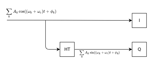
A real signal

$$ y(t) = \sum_{k} A_k \cos ((\omega_c + \omega_k) t + \phi_k) $$

is passed through a Hilbert transformer (which is a realization of the Hilbert Transform) to create a \(-\frac{\pi}{2}\) out of phase signal, which is the quadrature component. The I and Q components will describe an analytic signal

However, there are two issues:

• high frequency, broadband Hilbert transformers are hard to implement
• digital sampling and processing gets more difficult the higher the frequency, to the point it becomes impractical.

As a result, we usually perform mixing and I/Q conversion in succession, in order to address both issues. The following image describes a common real-to-I/Q mixer-converter combo, commonly called a quadrature mixer.

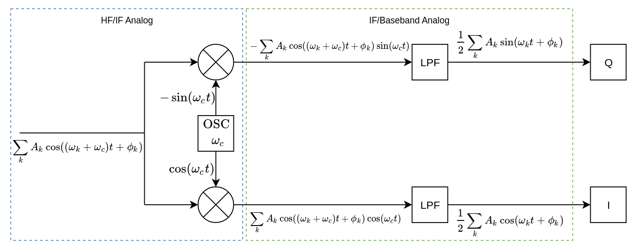
The real signal is fed into the module, which uses two frequency mixers and a complex oscillator \(c^\star(t) = e^{-j \omega_c t}\).

The in-phase mixer uses the in-phase (real) component of the oscillator, yielding the output:

$$ \begin{align} m_i(t) & = y(t) \Re e (c^\star(t)) \\ & = \sum_{k} A_k \cos ((\omega_c + \omega_k) t + \phi_k) \cos(\omega_c t) \\ & = \frac{1}{2} \sum_{k} A_k \cos (\omega_k t + \phi_k) + \frac{1}{2} \sum_{k} A_k \cos ((2 \omega_c + \omega_k) t + \phi_k) \end{align} $$

Then a low pass filter removes the high-frequency components from the mixer output:

$$ \begin{align} I(t) & = lpf(m_i(t)) \\ & = \frac{1}{2} \sum_{k} A_k \cos (\omega_k t + \phi_k) \end{align} $$

which generates the in-phase component of the output.

Transversely, something similar happens on the quardrature side:

$$ \begin{align} m_q(t) & = y(t) \Im m (c^\star(t)) \\ & = -\sum_{k} A_k \cos ((\omega_c + \omega_k) t + \phi_k) \sin(\omega_c t) \\ & = \frac{1}{2} \sum_{k} A_k \sin (\omega_k t + \phi_k) - \frac{1}{2} \sum_{k} A_k \sin ((2 \omega_c + \omega_k) t + \phi_k) \\ Q(t) & = lpf(m_q(t)) \\ & = \frac{1}{2} \sum_{k} A_k \sin (\omega_k t + \phi_k) \end{align} $$

which gives us the Q component of the output. The complex output can then be expressed as

$$ \begin{align} x^\star(t) & = I(t) + jQ(t) \\ & = \frac{1}{2} \sum_{k} A_k e^{j(\omega_k t + \phi_k)} \end{align} $$

This setup can be used either as an HF to IF downconverter, in which case the I and Q components are usually fed into an ADC, or as an IF to baseband or even HF to baseband downconverter, where the I/Q components can either be fed to an ADC or into an analog sideband selection module. Variations of this setup have the analog signals sampled right after the mixers, with the filtering performed digitally.

As opposed to the ideal converter discussed initially, the issue with this one is that the I/Q signal is clean only in the range \((-\omega_c, \omega_c)\); outside of this band we have aliasing. However, in practical applications \(\omega_c\) is large enough to accomodate any transmissions we desire.

On the other hand, an I/Q-to-real mixer may look like the following:

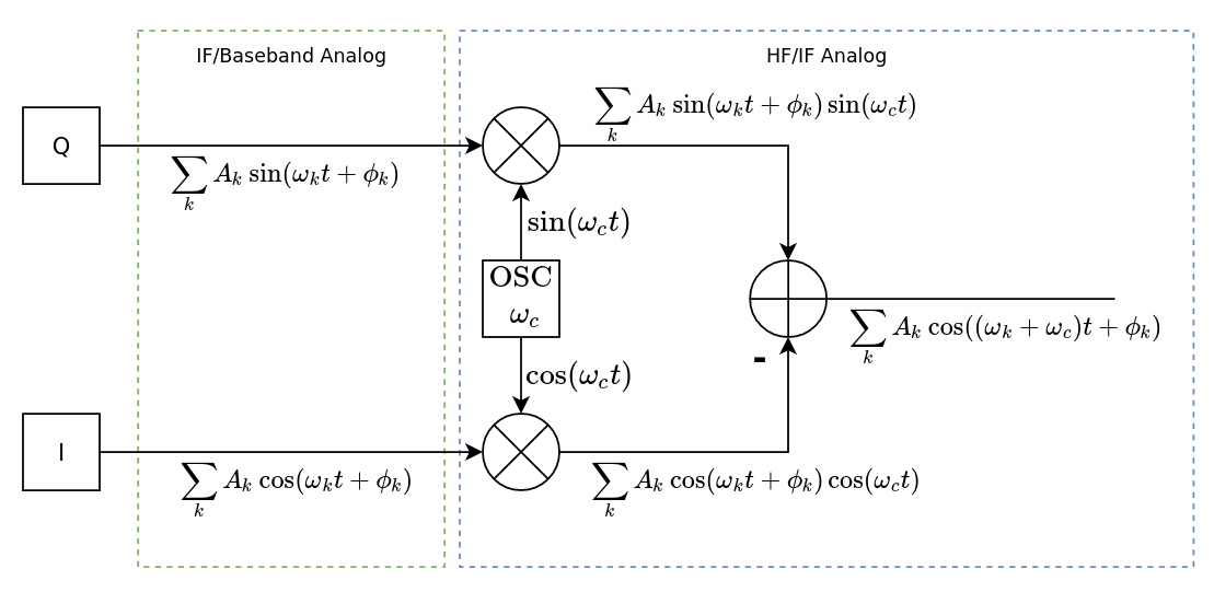
Given the complex signal \(x^\star\), the in-phase and quadrature mixer results are:

$$ \begin{align} m_i(t) & = \Re e (x^\star(t)) \Re e (c^\star(t)) \\ & = \sum_{k} A_k \cos (\omega_k t + \phi_k) \cos(\omega_c t) \\ & = \frac{1}{2} \sum_{k} A_k \cos ((\omega_k - \omega_c) t + \phi_k) + \frac{1}{2} \sum_{k} A_k \cos ((\omega_k + \omega_c) t + \phi_k) \ \ m_q(t) & = \Im m (x^\star(t)) \Im m (c^\star(t)) \\ & = \sum_{k} A_k \sin (\omega_k t + \phi_k) \sin(\omega_c t) \\ & = \frac{1}{2} \sum_{k} A_k \cos ((\omega_k - \omega_c) t + \phi_k) - \frac{1}{2} \sum_{k} A_k \cos ((\omega_k + \omega_c) t + \phi_k) \end{align} $$

The difference of these two signals will yield the real, single sideband signal:

$$ y(t) = m_i(t)-m_q(t) = \sum_{k} A_k \cos ((\omega_k + \omega_c) t + \phi_k) $$

Digital signal processing

Creating digital filters is much easier and more flexible that creating the analog counterparts from non-ideal discrete components like capacitors, inductors and resistors.

For example, in the analog domain, one would need to implement a bandpass filter for each and every bandwidth configuration of any supported modulation (e.g. AM, SSB, wide/narrow FM, CW, PSK etc). A digital signal processor can perform all this filtering and more, yet still have a physical footprint smaller than that of a capacitor. Moreover, filter characteristics can be configured on the fly, from user input, something that would be both difficult and expensive otherwise.

But what about modulation? It seems that, so far, we have looked at a very particular type of modulation (SSB-SC) which, while useful, seems rather limiting.

Well it turns out that the operation of frequency mixing a complex I/Q signal with an oscillator is sufficient to implement any kind of modulation.

Let’s take frequency modulation as an example, in which the frequency of a carrier wave is modulated by a baseband signal:

$$ \begin{align} y^\star_{FM}(t) & = e^{j(\omega_c + x(t))t} \\ & = e^{j \omega_c t} e^{j x(t) t} \\ & = c^\star(t) e^{j x(t) t} \end{align} $$

Phase modulation is even more straightforward:

$$ \begin{align} y^\star_{PM}(t) & = e^{j(\omega_c t + x(t))} \\ & = e^{j \omega_c t} e^{j x(t)} \\ & = c^\star(t) e^{j x(t)} \end{align} $$

DISCLAIMER: The above formulas are simplified versions of the actual modulations, but the point stands.

But, you say, I could have achieved this with real signals just as easily; complex signals don’t seem to be very useful for anything other than representation and filtration of negative frequencies.

And wrong you are. For example, PM demodulation is the retrieval of the phase from the complex signal, which as we’ve seen earlier is the polar coordinate of the geometric representation. Thus:

$$ \begin{align} x(t) & = \operatorname{atan2} \left ( sin(x(t)), cos(x(t)) \right ) \\ & = \operatorname{atan2} \left ( \Im m (e^{j x(t)}), \Re e (e^{j x(t)}) \right ) \\ & = \operatorname{atan2} \left ( \Im m \left ( y^\star_{PM}(t) \overline{c^\star(t)} \right) , \Re e \left ( y^\star_{PM}(t) \overline{c^\star(t)} \right) \right ) \\ & \text{for } x(t) \in (-\pi, \pi) \end{align} $$

Not to say that it wouldn’t be possible to perform this demodulation on a real signal, but it would have been considerably more difficult. And that’s the gist of it, in general most processing related to modulation and filtering of time-variant signals is easier to perform on their complex representation, especially when they are digital.

As a result, digital signal processing is the preferred method in today’s software-defined radio transceivers.