Today we aim to take a closer look at float, the ubiquitous data type we use whenever we’re forced to leave the discrete confines of integers. While a very flexible data type, it is not without its flaws, and we will explore a few of them further down.

We’ll start with a short crash course into the representation scheme of the floating point representation and then look at two real-world (but made up) scenarios any engineer may find himself or herself in one day.

Bear in mind this is not a definitive guide nor an in-depth analysis. Its only purpose is to open the door towards more complex topics.

A primer into the floating point representation

The IEEE-754 standard defines a representation that has a wider range (domain) than integers, but can also store and operate on rational numbers.

The representation splits the word into three parts:

• the sign bit \(s\)
• the exponent \(e\), stored internally as a \(b_e\)-bit unsigned integer
• the significand or coefficient \(c\), stored internally as a \(b_c\)-bit unsigned integer

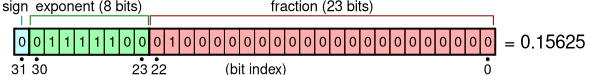
Depending on the word size, the coefficient and exponent may use various lengths; for example, \(32\)-bit floating point numbers have \(b_c=23\) and \(b_e=8\).

The mapping from state to value is:

$$ f(s, e, c) = (-1)^s \times 2^{e-2^{b_e-1}+1} \times (1 + c \times 2^{-b_c}) \\ \forall e \in { 1, 2, \dots 2^{b_e}-2 } \text{, } c \in { 0, 1, 2, \dots 2^{b_c}-1 } $$

As you can guess, the term \(1 + c \times 2^{-b_c}\) in the above formula is simply the binary number \( \overline{1.c_{22} c_{21} c_{20} … c_{0}} \), where \(c_i\) is the \(i\)-th bit of the coefficient \(c\); this term has the domain \([1.0, 2.0)\).

There are two special cases:

• \(e = 0\) codes subnormal numbers, values between \(\pm 0\) and the smallest possible normal numbers \(\pm 2^{-2^{b_e-1}+2}\)
• \(e = 2^{b_e}-1\) codes the values \(\pm \infty\) and \(NaN\)

The underlying difference between ints and floats

One of the most common misconceptions is that, for a given word size, the floating point representation has better precision than the integer representation. Overall both are coded into the same number of bits.

But how is this possible, since a float can store values as little as \(0.00001\) and as large as \(10^{25}\)?

Let’s look at the distribution of values over a large domain:

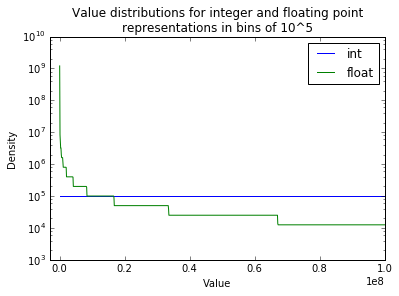
We can see that, while the representable integer values are uniformly distributed across the domain, the representable floating point values are not.

Looking at the map \(f\) it is obvious why. For any exponent \(e_k\), the interval of representable values has a uniform distribution; in other words, for \(32\)-bit floats the distance between any two successive values is equal to \(2^{e_k-127} \times 2^{-23}=2^{e_k-150} \).

However, once the coefficient is saturated, the successor of this value will take the exponent \(e=e_k+1\) and coefficient \(c=0\). The distance between all subsequent values will now be \(2^{e_k+1-150-23}=2^{e_k-149}\).

In conclusion, the distance between representable values doubles every time the coefficient saturates (that is, every \(2^{b_c}\) values). As a result, floats can have better precision and better range than integers, but it can’t do both at the same time.

Precision-wise, \(32\)-bit floats will outperform ints only between \(0\) and \(10^7\), which is less than \(1%\) of the \(32\)-bit integer domain.

Representation error

Since we are mapping a continuous domain (\(\Bbb{R}\)) to the discrete domain of representable floating point numbers, it follows that there will be some sort of approximation involved. While the IEEE-754 standard specifies multiple rounding modes, the most common is round-to-nearest, which simply maps the real value to the nearest representable value.

In order to better understand the process, we must define two kinds of errors. The absolute error

$$ \Delta x = |\hat{x} - x| $$

is simply the distance from the real (or true) value \(\hat{x}\) to the representable value \(x\). Hence, in round-to-nearest the representation function will output the \(x\) for which \(\Delta x\) is minimal.

But the absolute error is not a fitting metric for all scenarios; after all, it is much worse to be off by \(0.5m\) when we’re measuring \(2m\) than when we are measuring \(2km\). Thus, the relative error is defined as

$$ \frac{\Delta x}{|\hat{x}|} $$

and it measures how large the error is in comparison to the value being stored.

In order to see how \(\hat{x}\) maps to \(x\) and what the errors are, let’s write a positive \(\hat{x} \gt 0 \) in a friendlier form:

$$ \begin{align} \hat{x} & = 2^{\lfloor log_2 \hat{x} \rfloor} \times \hat{x} \times 2^{- \lfloor log_2 \hat{x} \rfloor} \\ & = 2^{\lfloor log_2 \hat{x} \rfloor} \times (1 + \hat{x} \times 2^{- \lfloor log_2 \hat{x} \rfloor} - 1) \\ & = 2^{\lfloor log_2 \hat{x} \rfloor} \times \left ( 1 + \left (2^{23} \times ( \hat{x} \times 2^{- \lfloor log_2 \hat{x} \rfloor} - 1) \right ) \times 2^{-23} \right ) \end{align} $$

NOTE: \(\lfloor log_2 x \rfloor\) was chosen because \( x \times 2^{-\lfloor log_2 x \rfloor} \in [1, 2) \).

It is now easy to identify the integer exponent and coefficient of a \(32\)-bit floating point representation:

$$ \begin{align} e & = \lfloor log_2 \hat{x} \rfloor + 127 \\ c & = \lfloor 2^{23} \times (\hat{x} \times 2^{- \lfloor log_2 \hat{x} \rfloor} - 1) \rceil \end{align} $$

So then the map will be

$$ \begin{align} x & = 2^{e -127} \times (1 + c \times 2^{-23}) \\ & = 2^{\lfloor log_2 \hat{x} \rfloor} \times \left ( 1 + \lfloor 2^{23} \times (\hat{x} \times 2^{- \lfloor log_2 \hat{x} \rfloor} - 1) \rceil \times 2^{-23} \right) \\ & = 2^{\lfloor log_2 \hat{x} \rfloor} \times \left ( 1 + \lfloor \hat{x} \times 2^{23- \lfloor log_2 \hat{x} \rfloor} - 2^{23} \rceil \times 2^{-23} \right) \\ & = 2^{\lfloor log_2 \hat{x} \rfloor -23} \times \left \lfloor \hat{x} \times 2^{23- \lfloor log_2 \hat{x} \rfloor} \right \rceil \end{align} $$

and the representation absolute error

$$ \begin{align} \Delta x & = |\hat{x} -x| \\ & = \left | \hat{x} - 2^{\lfloor log_2 \hat{x} \rfloor - 23} \times \left \lfloor \hat{x} \times 2^{23 - \lfloor log_2 \hat{x} \rfloor} \right \rceil \right | \\ & = 2^{\lfloor log_2 \hat{x} \rfloor - 23} \times \left ( \left | \hat{x} \times 2^{23 - \lfloor log_2 \hat{x} \rfloor} - \left \lfloor \hat{x} \times 2^{23 - \lfloor log_2 \hat{x} \rfloor} \right \rceil \right | \right ) \end{align} $$

Since

$$ | k - \lfloor k \rceil | \le 2^{-1} \text{, } \forall k \in \Bbb{R}_{+} $$

we can find the non-optimal (but good enough) representation absolute error upper bound

$$ \Delta x \le 2^{\lfloor log_2 \hat{x} \rfloor - 24} \le \hat{x} \times 2^{-24}$$

and the representation relative error upper bound

$$ \frac{\Delta x}{|\hat{x}|} \le 2^{-24} \approx 6e-8 $$

which is also called the machine epsilon.

Thus, we can observe that the floating point representation has an absolute error fairly proportional to the value (which we could have guessed from the previous distribution plot), but more importantly has a fairly constant relative error.

In other words, any \(32\)-bit floating point value can’t be more than \(0.000006 %\) off from the true value.

Floating point decimal precision

An important observation is that the floating point representation is a binary representation. As a result it guarantees storage of \(b_c\) significant binary digits, which do not necessarily correlate to decimal digits.

For example:

• the number \(0.0078125\) is perfectly representable (i.e. has zero representation error), since it can be written as \(2^{-7} \times 1.0\)
• the number \(0.1\) is represented in \(32\)-bit floats as \(0.10000000149011612 \dots \), since it cannot be written as a finite sum of powers of two

In conclusion, it is not a good idea to gauge the representation error by the number of significant decimal digits.

NOTE: The latest revision of the IEEE-754 standard actually defines new decimal floating point formats. Since hardware support for them is virtually non-existent we can safely ignore them for the time being.

The problem of docking spacecrafts

Let’s say we’re writing the guidance software for a spacecraft that is to leave Earth orbit, inject into a Martian orbit and dock with another craft that is already there.

Since we’re dealing with more than one planet, we build a heliocentric model of our solar system, at the heart of which is the orbital prediction function \(O_p\), which outputs the craft position relative to the primary body (i.e. Earth, Mars, Sun) given a set of orbital parameters and a time value.

Then, given the Martian orbital parameters \(\gamma_m\), target craft’s orbital parameters \(\gamma_t\), our craft’s primary body orbital parameters \(\gamma_{pri}\), and our craft’s orbital parameters \(\gamma_s\), we have the absolute position of the two crafts at some point in time \(t\):

$$ p_t (t) = O_p(\gamma_m, t) + O_p(\gamma_t, t) \\ p_s (t) = O_p(\gamma_{pri}, t) + O_p(\gamma_s, t) $$

Since docking is a fiddly operation, we want to compute ahead of time the moment of rendezvous, or the time when the distance between two spacecrafts is minimal. We define the distance between the two crafts:

$$ d(t) = \lVert p_t(t) - p_s(t) \rVert $$

for which we need to find

$$ t_{r} = \arg \min_{t} d(t) $$

for \(\gamma_{pri} = \gamma_m\), which we compute numerically by evaluating \(d(t)\) for sufficiently many \(t\).

Our code might look like the following:

def Op(orbit_params, t):
    # assume perfect implementation

def get_target_abs_position(t):
    return Op(mars_orbit_params, t) + Op(target_orbit_params, t)

def get_spacecraft_abs_position(pri_orbit_params, t):
    return Op(pri_orbit_params, t) + Op(spacecraft_orbit_params, t)

def get_abs_distance(pri_orbit_params, t):
    return np.norm(get_target_abs_position(t)
                   - get_spacecraft_abs_position(pri_orbit_params, t))

def get_rendezvous_time():
    d_min = +inf
    for t in np.linspace(now(), now() + 2days, 1000000):
        d = get_abs_distance(mars_orbit_params, t)
        if d < d_min:
            d_min = d
            t_r = t
    return t_r, d_min

Then the moment comes when we perform the final burn, we compute \(\gamma_s\), make the call to get_rendezvous_time and observe that we will perfectly intercept the target spacecraft. We take out the champagne and celebrate!

Then \(t_r\) comes and goes, and there’s no sign of the other craft.

Loss of significance

What happened? We nervously start debugging the code, looking for the flaw that just lost us a few billion dollars.

It can’t be Op, we’ve used this code to compute sattelite positions for some time now.

It can’t be get_spacecraft_abs_position or get_target_abs_position, we’ve used them to compute communication round-trip-time, and it was always on point.

It can’t be the floating point representation, since we know it behaves well due to its very low relative error. Or does it?

The truth is all the code is correct, but we just suffered a case of loss of significance under subtraction, or (very fittingly) catastrophic cancellation.

The issue was our misunderstanding of the low relative error of the floating point representation. While individually each operation is safe in relation to it’s output, it may not be in relation to the target quantity.

Let’s look to a unidimensional scenario of our algorithm for some \(t\). The table contains the actual result of the operation in \(32\)-bit floating point representation, the mathematical result of the operation (applied on operators), the relative error of the operation and the true result (evaluated in a perfect representation).

$$ \begin{array}{|c|c|c|c|c|} \hline \text{Operation} & \text{Operation} & \text{Mathematical} & \text{Relative} & \text{True} \\ x & \text{result }(x) & \text{result } (x^*) & \text{error} & \text {result } \hat{x} \\ \hline O_p(\gamma_m, t) & 227900000km & 227900000km & 0.0 & 227900000km \\ \hline O_p(\gamma_t, t) & 12334.595703km & 12334.596km & <10^{-7} & 12334.596km \\ \hline O_p(\gamma_s, t) & 12334.318359km & 12334.318km & <10^{-7} & 12334.318km \\ \hline p_t(t) & 227912336km & 227912334.595703km & <10^{-8} & 227912334.596km \\ \hline p_s(t) & 227912336km & 227912334.318359km & <10^{-8} & 227912334.318km \\ \hline d(t) & 0.0km & 0.0km & \text{N/A } (0) & 0.278km \\ \hline \end{array} $$

We managed to compute the positions of the target \(O_p(\gamma_t, t)\) and the spacecraft \(O_p(\gamma_s, t)\) with absolute errors of less than a meter. However, the problem rears its head when we compute the absolute positions \(p_t(t)\) and \(p_s(t)\); while they have very low relative errors, the absolute errors are comparable to the quantity we are measuring (distance between crafts). Thus, while the evaluation of \(d\) has zero error by itself, the error compounded in the operands has a destructive effect on our computation.

Obviously, any of the two computed distances would be perfectly fine if we were evaluating radio round-trip-time \(rtt = \frac{p_s(t)}{c}\), since \(rtt\) is the measured quantity and the relative error is computed with respect to it. In fact even \(d(t)\) may have had a perfectly acceptable error had our spacecraft been orbiting Earth, since our focus would not have been docking, but some other metric at a planetary scale.

To summarize, our problem is that we are asking for too great a precision for the domain we are operating on.

In order to fix such problems, we always look at the mathematical model and find an equivalent form in which the discrepancy between the operand domains and measurement domain is reasonable. If we take the function \(d\) that we minimize, and specialize it for \(\gamma_{pri} = \gamma_m\) we get:

$$ \begin{align} d(t) & = \lVert p_t(t) - p_s(t) \rVert \\ & = \lVert O_p(\gamma_m, t) + O_p(\gamma_t, t) - O_p(\gamma_{pri}, t) - O_p(\gamma_s, t) \rVert \\ & = \lVert O_p(\gamma_t, t) - O_p(\gamma_s, t) \rVert \end{align} $$

which is perfectly intuitive, since there is no need to compute the absolute positions of the crafts given they orbit the same body. In consequence, we now get a numerical result of \(d = 0.277344km\), which is much closer to the true value of \(\hat{d} = 0.278km\).

Obfuscation by good coding practice

Not all scenarios are as nicely laid out for us as this tought experiment, and it is sometimes difficult to identify potential sources of loss of significance.

Mathematical models are often expressed in a form that is easiest for humans to comprehend, but which can otherwise be numerically unstable under finite representations.

Moreover, when working with implementations of such models, it is very tempting and often encouraged to use existing functionality (like the functions get_*_abs_position in our examples) instead of implementing a specialization for our use case.

But above all, it is not necessary to be a rocket scientist to feel the effects of numerical errors, as we will see in the next sections.

The problem of the power meter

We’ve obviously been fired from our job as a rocket scientist, and we’re now demoted to writing firmware for power meters.

Our taks is to measure a household’s power consumption over a large period of time. In order to achieve this, we have a power transducer that measures the instantaneous power consumption and outputs a DC voltage in the \(0-5V\) range, corresponding to the measurement domain of \(0-5kW\). The DC voltage is translated by an ADC to a floating point number equal to the input voltage.

Since it is a trivial problem, we implement a trivial solution:

def power_meter_main_loop():
    reading_freq_hz = 10
    usage = load_usage_from_storage()
    while True:
        usage += adc_read()
        usage_kwh = usage / (reading_freq_hz * 3600)
        display(usage_kwh)
        save_usage_to_storage(usage)
        sleep(1 / reading_freq_hz)

We choose a sampling frequency of \(10Hz\) for our device and, at each iteration, we read a value from the ADC and accumulate it to usage. Since usage is expressed in \(kW \cdot ds\) (kilowatt-decisecond), we need to convert it to \(kW \cdot h\) and display it on the power meter’s LCD. We also save our usage to a non-volatile memory so we can retrieve it in case of a power outage.

The power meter gets released into production, installed in many homes and everything looks great. We take out the champagne and celebrate!

Then one year later, the company stops making any money. Crap…

Vanishing values

Weirdly enough, all power meters seem to have stopped at \(3728.27 \text{ } kW \cdot h\), and all tests on the hardware indicate that it is working properly. It then must be a software bug.

Since the \(kW \cdot h\) is only used for displaying the value, we compute the underlying accumulator value of \(134217728.0 \text{ } kW \cdot ds\).

As it happens, this value is a power of two, \(2^{27}\) to be precise. The question is now, why is this an upper bound for our accumulator?

Let’s consider two representable, positive, \(32\)-bit floating point values

$$ x_1 = 2^{e_1-127} (1 + 2^{-23}c_1) \\ x_2 = 2^{e_2-127} (1 + 2^{-23}c_2) $$

where \(e_1, e_2, c_1, c_2 \in \Bbb{N} \text{, } c_1, c_2 \lt 2^{23} \).

Let’s try to find the representation \(y = 2^{e_y-127} (1 + 2^{-23}c_y)\) of \(x_1+x_2\).

If \(x_1 \ge x_2\) we can compute the true value as

$$ \begin{align} \hat{y} & = x_1 + x_2 \\ & = 2^{e_1-127} (1 + 2^{-23}c_1) + 2^{e_2-127} (1 + 2^{-23}c_2) \\ & = 2^{e_1-127} \left ( 1 + 2^{-23}c_1 + 2^{e_2-e_1} (1 + 2^{-23}c_2) \right ) \\ & = 2^{e_1-127} \left ( 1 + 2^{-23}(c_1 + 2^{e_2-e_1}c_2 + 2^{23+e_2-e_1}) \right ) \end{align} $$

But since \(y\) must also be representable, then it follows that \(c_y \in \Bbb{N}\), so then

$$ c_y = \lfloor c_1 + 2^{e_2-e_1}c_2 + 2^{23+e_2-e_1} \rceil $$

Interestingly enough, if \(e2-e1 \le -25\), then

$$ 2^{e_2-e_1}c_2 \lt 2^{-2} \\ 2^{23+e_2-e_1} \le 2^{-2} $$

so it follows that

$$ 2^{e_2-e_1}c_2 + 2^{23+e_2-e_1} \lt 2^{-1} \\ \lfloor 2^{e_2-e_1}c_2 + 2^{23+e_2-e_1} \rceil = 0 $$

Since \(c_1 \in \Bbb{N}\) it follows that \(c_y = c_1\), and since \(e_y = e_1\) then \(y = x_1\).

We can conclude that if there is a difference of more than 24 between the exponents of two values, then their sum will always evaluate to the larger of them. Or, if we translate to decimal, if there is a difference of about seven or more orders of magnitude between the two operands, the sum will evaluate to the larger of them.

Now let’s see what happened in our scenario; we have our accumulator \(2^{27}\) with \(e_a = 27+127=154\), and the maximum value of the sample \(5.0\) with \(e_s = \lfloor \log_2 5 \rfloor + 127 = 2+127=129 \).

Since \(e_a - e_s \ge 25\) we can conclude that it would be technically impossible for the power meter to overcome this value, since any possible summation would simply evaluate to the accumulator value.

Manifestation of the same underlying issue

Intrinsically we have the same issue as with the spacecraft example, with the distinction that instead of the result having a much smaller domain than both operands, one of the operands has a much smaller domain the the other and the result.

In fact, the above scenario is an extreme manifestation of a loss of precision due to large domain discrepancies (where \(\frac{x_2}{x_1}\) approaches machine epsilon). In actuality, the power meter’s performance started slowly degrading the moment it was turned on.

If we look at the sum’s representation, we see that

$$ \begin{align} c_y & = \lfloor c_1 + 2^{e_2-e_1}c_2 + 2^{23+e_2-e_1} \rceil \\ & = c1 + \lfloor 2^{e_2-e_1}(c_2 + 2^{23}) \rceil \end{align} $$

Thus, the actual representable value we add to the accumulator during each summation is

$$ x_2’ = 2^{e1-104} \lfloor 2^{e_2-e_1}(c_2 + 2^{23}) \rceil $$

Then, the error relative to \(x_2\) is

$$ \begin{align} \frac{|x_2 - x_2’|}{|x_2|} & = \left | 1 - \frac{x_2’}{x_2} \right | \\ & = \left | 1 - \frac{2^{e1-104} \lfloor 2^{e_2-e_1}(c_2 + 2^{23}) \rceil}{2^{e_2-127} (1 + 2^{-23}c_2)} \right | \\ & = \left | 1 - \frac{2^{e1-104} \lfloor 2^{e_2-e_1}(c_2 + 2^{23}) \rceil}{2^{e1-104} \times 2^{e_2-e_1}(c_2 + 2^{23})} \right | \\ & = \left | 1 - \frac{\lfloor 2^{e_2-e_1}(c_2 + 2^{23}) \rceil}{2^{e_2-e_1}(c_2 + 2^{23})} \right | \end{align} $$

We can parametrize for \(\Delta e=e_1-e_2\):

$$ \frac{|x_2 - x_2’|}{|x_2|} = \left | 1 - \frac{\lfloor 2^{-\Delta e}(c_2 + 2^{23}) \rceil}{2^{-\Delta e}(c_2 + 2^{23})} \right | $$

and compute the mean error relative to \(x_2\) for any \(\Delta e\) as

$$ M_e(\Delta e) = \frac{1}{2^{23}} \sum_{c2 = 0}^{2^{23}-1} \left ( \left | 1 - \frac{\lfloor 2^{-\Delta e}(c_2 + 2^{23}) \rceil}{2^{-\Delta e}(c_2 + 2^{23})} \right | \right ) $$

Thus the value of \(M_e(\Delta e)\) is the mean relative error of the information we are trying to inject into the accumulator for an exponent difference of \(\Delta e\). Or in the general case, the mean error of the floating point addition relative to the smaller operand, for an exponent difference of \(\Delta e\).

While the above can be computed analitically, we are interested only in its graph:

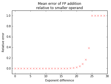
We can clearly see the behaviour we determined in the previous section, where all information is lost for \(\Delta e \ge 25\).

But more relevant is the relationship between the above relative error and the accumulator iteration:

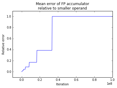
As we can see, the error relative to \(x_2\) increases somewhat linearly with the iteration number, until \(\Delta e = 25\) is reached. As a result, before the failure, the power meter functioned for more than \(80%\) of its life with an unacceptably high error.

Fixes

A more fitting representation for an accumulator is the integer representation, since it has a constant absolute representation error and zero error over addition, subtraction and multiplication.

If for some reason there is a hard constraint for a floating point representation, then there are some solution’s like Kahan’s algorithm that mitigates this error.

Epilogue

We’ve barely scratched the surface of the types of issues we can encounter when performing arithmetic on finite representations - there is actually a whole field of mathematics called numerical analysis that deals with this.

But what I hope we can take from this text is the intuition of where the important information is coded in our algorithm and how it is handled by the representation. We may not always have the time to find the optimal solution, nor to perform an exhaustive analysis on our model, but what is important is that we do not mess up too badly.